Daily ETF RSI-MA Bot on Quantconnect

Hourly swing-trader with momentum fallback

Scans the 20 most-liquid US ETFs each hour, buys when RSI rebounds from oversold and the 50-hour MA sits above the 200-hour MA. If nothing is oversold, it falls back to a simple 30-day momentum rank so it never stands idle. Risk is allocated by inverse ATR and capped at 2 × gross exposure.

Core Parameters

# look-back & thresholds
rsiPeriod        = 14
fastPeriod, slowPeriod = 50, 200   # hourly SMA trend filter
oversold, overbought   = 30, 70

# risk & exits
stopATR  = 1.5      # initial stop
trailATR = 1.5      # trailing once in profit
holdMaxHrs, earlyExitHrs = 48, 32
earlyExitATR = 0.5   # bail if no progress
targetExposure = 2.0 # 2× gross cap

These numbers aim for frequent trades but shallow risk— a 1½ × ATR stop is tight on purpose to keep max drawdown low.

Universe → keep it liquid

def CoarseSelection(self, coarse):
    liquid = [c for c in coarse
              if c.Symbol.Value in self.etfCandidates
              and c.DollarVolume > 25e6]           # ≥ $25 M / day
    return [c.Symbol for c in sorted(liquid,
                                     key=lambda x: x.DollarVolume,
                                     reverse=True)[:30]]

Anything thinner than $25 M daily volume is skipped to avoid sloppy spreads and halts.

Risk-On Regime Check

self.spyFast = self.SMA('SPY', 50, Resolution.Hour)
self.spySlow = self.SMA('SPY', 200, Resolution.Hour)

riskOn = self.spyFast.Current.Value > self.spySlow.Current.Value

The bot only opens new trades when SPY’s short MA is above its long MA—keeps it out of bear swoons.

Entry: RSI swing-reversal

longSetup = (rsi < 30) and (rsi > prevRsi)        # ticking up
trendUp   = sma50 > sma200
if riskOn and longSetup and trendUp:
    self.SetHoldings(sym, +weight)

• Mirror logic for shorts when RSI > 70 plus down-trend.
• If no ETF is oversold/overbought, the bot looks at price momentum over the past 30×7 bars:

hist = self.History(sym, 210, Resolution.Hour)
momentum = (price - hist.close.iloc[0]) / hist.close.iloc[0]

Sizing: inverse-ATR

invVol[sym] = 1 / atrValue
w = invVol[sym] / Σ(invVol) * targetExposure   # <= 2× gross

Quiet ETFs (low ATR) get bigger weights; choppy ones get trimmed so each position risks roughly the same euro amount.

Exit rules

stop  = entry - 1.5 * ATR
trail = price - 1.5 * ATR   # only ratchets higher
if heldHrs >= 32 and price < entry + 0.5 * ATR:
    self.Liquidate(sym)     # early exit (no progress)
if heldHrs >= 48:
    self.Liquidate(sym)     # hard time-stop

Stops trail by the same ATR multiple to keep risk constant as a trade moves.

How one hour flows

Every hour: update indicators → score momentum → size positions → log to QC.

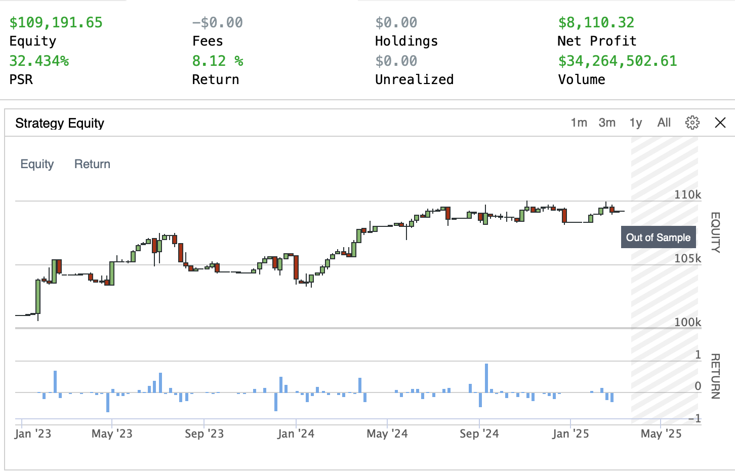
Back-test detail

• Win rate: 47 %
• Profit-loss ratio: 1.32
• Expectancy: 0.10 R per trade
• Turnover: ≈ 40 % of the book per year
• Fees: $0 (Alpaca sim)

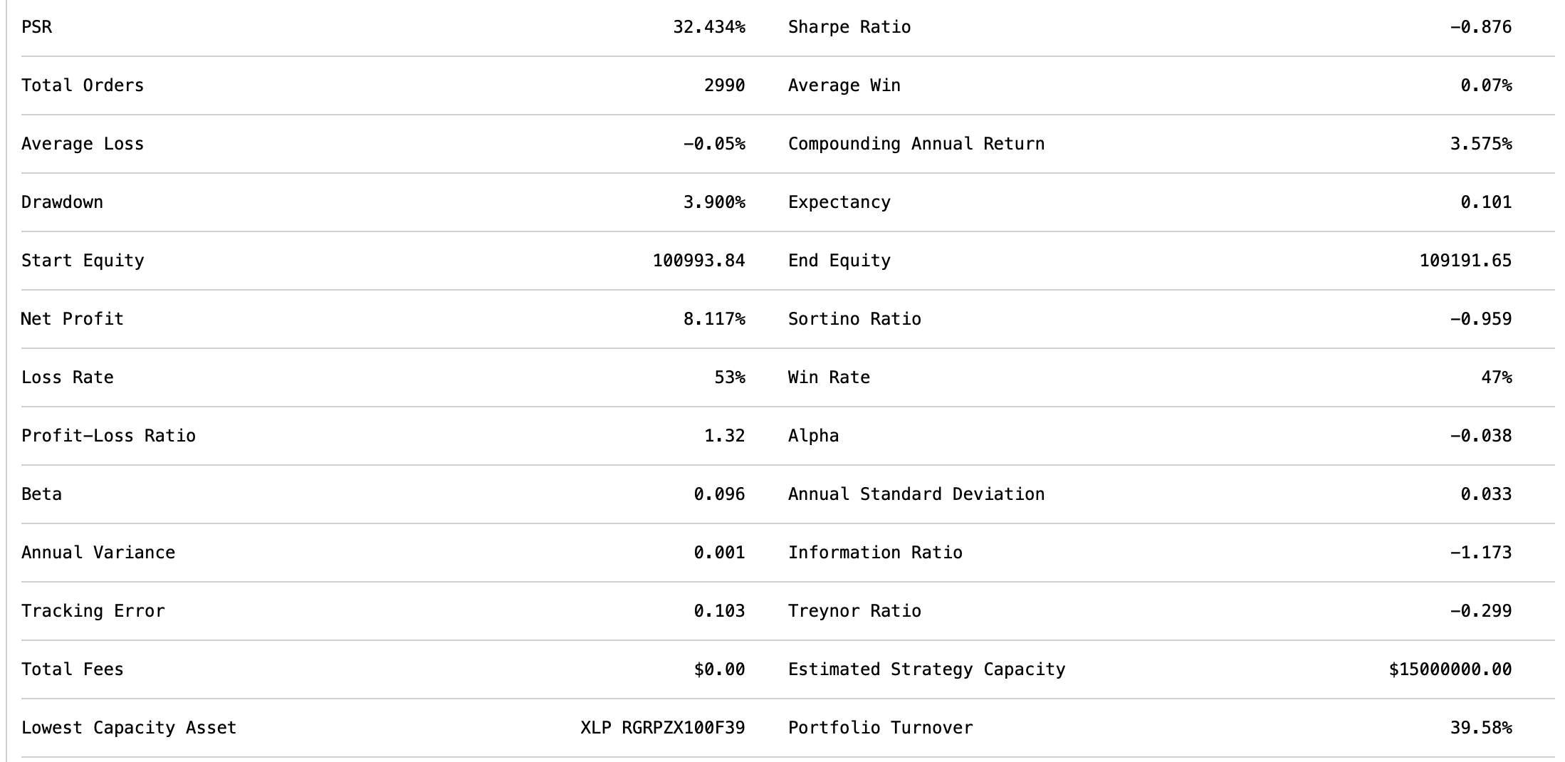
Stats exported from QuantConnect run “Well Dressed Sky Blue Tapir”

Next → Iteration ideas

1. Pause short-selling when VIX < 15 (fade traps).
2. Add a > 2 × ATR gap filter to skip blow-outs at the open.
3. Rolling 20-day Sharpe guardrail → auto-suspend on 3 σ slumps.
4. Stream logs to FastAPI for near-real-time PnL dashboards.

Building this bot was genuinely fun—every tweak taught me something new about Lean and market micro-behaviour. I’m definitely going to sink more evenings into refining these edges! :)